adding_to

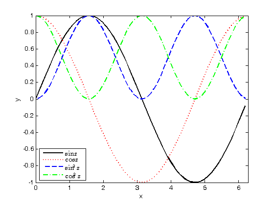
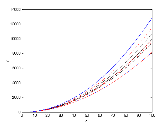
% Jake Bobowski
% August 18, 2017
% Created using MATLAB R2014a

% This tutorial demonstrates how to successively add curves and/or data to
% a single plot.

clearvars

% In basic_plots.m, we say that it was easy to put multiple curves on a
% single plot by specifying multiple functions in a single plot command.
% For example:
xx = 0:0.1:2*pi;
plot(xx, sin(xx), 'k-', xx, cos(xx), 'r:', 'LineWidth', 2)
xlabel('x')
ylabel('y')
axis([0 2*pi -1 1])

% What if we now wanted to add a third curve to our plot?  If we make a new
% plot command right now, it will overwrite the previous plot.  In MATLAB,
% if the statement 'hold on' is used between plot statements, the new
% curves will be added to previous plots.  For example:
hold on;
plot(xx, sin(xx).^2, 'b--', 'LineWidth', 2)

% Once the 'hold on' statement has been executed, we can continue to add
% to our existing plot.  Let's also add a legend to the plot.
plot(xx, cos(xx).^2, 'g-.', 'LineWidth', 2)
legend({'$\sin x$', '$\cos x$', '$\sin^2 x$', '$\cos^2 x$'}, 'Interpreter', 'LaTeX', 'location', 'southwest')

% Once we're done adding stuff to this plot, we execute 'hold off'.
hold off;

% If we were now to write another plot command it would overwrite the plot
% that we just finished creating.  To avoid doing that, we should use
% 'figure()' to start a new window before making the next plot.
figure();

% Using a for loop and 'hold on', we can easily add many curve to a single
% plot.  In the loop below, normrnd(mu, sigma) is used to generate random
% numbers drawn from a normal distribution with mean mu and standard
% deviation sigma.
xx = 0:1:100;
plot(xx, xx.^2, 'k-')
xlabel('x')
ylabel('y')
format = {'k--', 'k:', 'k-.', 'r-', 'r--', 'r:', 'r-.', 'b-', 'b--', 'b:'};
hold on;
for i = 1:10
    mu = 2;
    sigma = 0.05;
    n = normrnd(mu,sigma);
    plot(xx, xx.^n, format{i});
end
hold off;