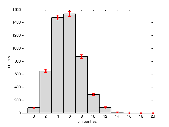
% Jake Bobowski
% August 18, 2017
% Created using MATLAB R2014a

% This tutorial demonstrates shows how to create histograms in MATLAB.

clearvars

% First, we create a vector of 5,000 random numbers drawn from a Poisson
% distribution.
mu = 6;
for i = 1:5000
    n(i) = poissrnd(mu);
end

% A histogram can be created simply using 'hist(n)'.
% **IMPORTANT** MATLAB says that 'hist' is no longer recommended.  They
% suggest using 'histogram' instead.  However, 'histogram' does not seem
% to work in MATLAB 2014a (which I am currently using).  If you are working
% with a newer version of MATLAB, you may want to try using 'histogram' in
% place of 'hist'.
hist(n);
xlabel('bin centres')
ylabel('counts')

% I don't understand it, but I looked up how to change to colour of the
% bars in the histogram.  For what it's worth, here's what I found:
figure();
hist(n);
xlabel('bin centres')
ylabel('counts')
set(get(gca, 'child'), 'FaceColor', 'y', 'EdgeColor', 'c', 'LineWidth', 2);

% Rather than having hist decide for you, you can specify the number of
% bins used to generate the histogram.
figure();
nbins = 12;
hist(n, nbins);
xlabel('bin centres')
ylabel('counts')
set(get(gca, 'child'), 'FaceColor', 'm', 'EdgeColor', 'k', 'LineWidth', 2);

% Instead of specifying the number of bins, you can provide a list of the
% bin centres.  Notice that I can also specify colours using RGB (red,
% green, blue) format.  I also called the histogram 'h'.
figure();
xbins = [0:2:20];
hist(n, xbins)
xlabel('bin centres')
ylabel('counts')
axis([-2 20 0 1600])
set(get(gca, 'child'), 'FaceColor', [0.85, 0.85, 0.85], 'EdgeColor', 'k', 'LineWidth', 2);

% It's worth noting that you can get vectors of the counts in each bin and
% the positions of the bin centres of a histogram using:
[counts, centres] = hist(n, xbins)

% You can also get the bin counts using 'histc'.  However, histc is bizarre
% in that, to get an aswer that agrees with 'counts' from above, we have to
% pass histc the positions of the bin edges, not the bin centres!
histc(n, -0.5:2:20.5)
% Whatever... it's probably best to just avoid histc altogether.

% Now that we have the counts and the bin centres we can, if we want, add a
% scatter plot to our histogram.  In fact, I chose a Poisson distribution
% at the beginning of this script because it arises in counting experiments
% and we know that for Poisson distributions the error in the number of
% counts in a bin is just the square root of the number of counts.
% Hold on...
hold on;
errorbar(centres, counts, sqrt(counts), 'r.', 'MarkerSize', 16, 'LineWidth', 1.5)
hold off;

% Here's a way to display multiple histograms in a single plot.
figure();
for j = 1:3
    for i = 1:2000
        m(i, j) = poissrnd(mu);
    end
end
hist(m, 0:4:20)
xlabel('bin centres')
ylabel('counts')
axis([-2 20 0 1200])

% Finally, we note that you sometimes may want to normalize your histogram
% so that you can put a pdf (Probability Density Function, not Portable
% Document Format) on top of it.  The probability that an event falls
% within a particular bin is given by the number of counts in that bin
% (after many many trials), divided by the total number of trials, or the
% total number of counts in all bins.  Remember, however, that we want to
% plot a probability density.  That is, we want to plot the probability per
% unit x, where x represents whatever quantity is plotted along the x-axis
% of the histogram.  To get a probability density, we must divide the
% number of counts in each bin by the product of the total number of counts
% and the bin width.
pdfData = counts/(sum(counts)*(xbins(2) - xbins(1)));

% We do an easy check to see if we've done things properly.  The itegral of
% our pdfData should equal one.  The integral can be approximated as...
sum(pdfData)*(xbins(2) - xbins(1))
% ... and we get a good result.

% Now we can make a new, normalized, histogram.  This time, we'll use 'bar'
% to make our histogram because we no longer have a list of random numbers
% that hist wants to use to bin the data an so on.
figure();
H = bar(xbins, pdfData, 'FaceColor' , 'y', 'EdgeColor', 'k', 'LineWidth', 2);
xlabel('bin centres')
ylabel('counts')
axis([-2 20 0 0.18])

% We can now add to this plot the expected Poisson pdf using the known mean
% of mu = 6 (look way back to the top of this script, line 11).  We use
% 'poisspdf' to calculate the Poission pdf at the bin centres.  Note that
% the Poisson distribution is a discrete distribution.  That is, it is only
% defined for integer values of x.  If you try to feed poisspdf noninteger
% x-values it will assign zero to the pdf at those values.
hold on;
y = poisspdf(xbins, mu);
plot(xbins, y, 'bx', 'LineWidth', 2, 'MarkerSize', 10);

% While poisspdf is technically correct for only outputting nonzero values
% at integer x-values, you may, perhaps, wish to show a continuous
% representation of the Poisson pdf for aesthetic reasons. Fortunately for
% you, some fine members of the MATLAB community has created and shared a
% function written to do just that.  It's called 'poisson.m'.  To use it,
% it must be located in the same directory as the script you're using to
% call the function.
xx = 0:0.01:30;
yy = poisson(xx, mu);
plot(xx, yy, 'b-', 'LineWidth', 1.5);
% So, finally, the above bar graph is our randomly generated Poisson
% distribution after it has been scaled to represent a probability density
% function (pdf).  The points represent the true (discrete) Poisson pdf
% using a mean of mu = 6.  The line is a continuous representation of the
% Poisson pdf.

hold off;

counts =

  Columns 1 through 6

          83         649        1477        1531         873         285

  Columns 7 through 11

          88          14           0           0           0


centres =

     0     2     4     6     8    10    12    14    16    18    20


ans =

  Columns 1 through 6

          83         649        1477        1531         873         285

  Columns 7 through 11

          88          14           0           0           0


ans =

     1

Published with MATLAB® R2014a