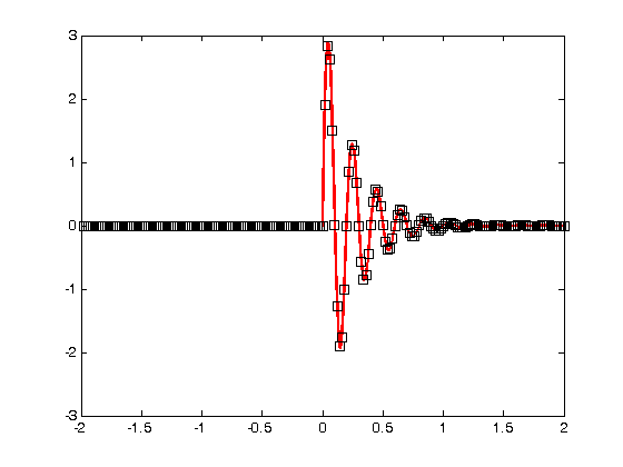
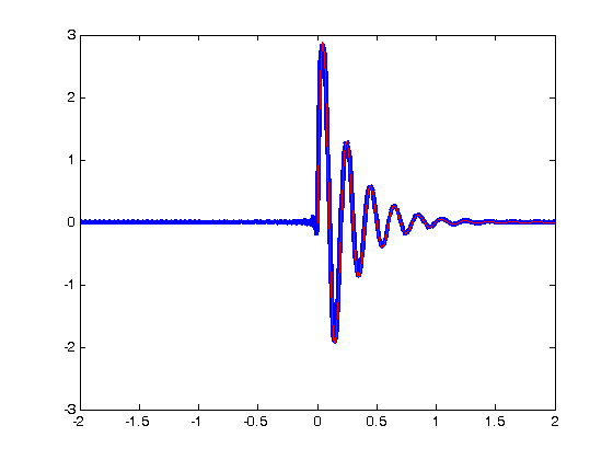
% Jake Bobowski
% March 1, 2018
% Created using MATLAB R2014a

% In this MATLAB tutorial we start with a cntinuous function of time from
% which we draw samples at a uniform sampling rate.  The sampling rate is
% chosen to be higher than the maximum appreciable frequency component
% contained in the original function of time.  We then attempted to
% reconstruct the original continuous function from the sampled data.

clearvars

% Here's the original function from which samples will be drawn.
ts0 = linspace(0, 2.5, 1000);
T = 0.2;
tau = 0.25;
A = 3.5;
f = A*sin(2*pi*ts0/T).*exp(-ts0/tau);
plot(ts0,f, 'r-', 'LineWidth', 2)
axis([-2 2 -3 3])


% Now do the sampling.  There are Ns samples between -tmax and +tamx.
% Therefore the time between samples is 2*tmax/(Ns - 1), or the sample
% frequency is (Ns - 1)/(2*tmax).
Ns = 1001;
tmax = 10;
ts = linspace(-tmax, tmax, Ns);
ys = A*sin(2*pi*ts/T).*exp(-ts/tau);
for i = 1:Ns
    if ts(i)<0
    ys(i) = 0;
    end
end;

% Plot the samples on top of the original continuous function.
hold on;
plot(ts, ys, 'ks')
hold off;

% Start a new figure.
figure;

% Define a variable (time).
syms t

% Here again are the sampling period and frequency.
Ts = ts(2)-ts(1);
fs = 1/Ts;

% This function will become the reconstructed signal.
yRe = @(t) 0;

% Let's do the reconstrcution using the sinc function!
set(0,'RecursionLimit',2000)
for i = -(Ns-1)/2:(Ns-1)/2
    n = i + (Ns-1)/2 + 1;
    yRe = @(t) yRe(t) + ys(n)*sin(pi*fs*(t-i*Ts))./(pi*fs*(t-i*Ts));
end

% Now make some time values and plot the reconstructed signal.
tt = linspace(-2.5, 2.5, 1000);
plot(tt, yRe(tt), 'b-', 'LineWidth', 3)
axis([-2 2 -3 3])

% Plot the original continuous function on top of the reconstructed signal
% to facilitate easy comparison.
hold on;
plot(ts0,f, 'r-', 'LineWidth', 0.5)
hold off;