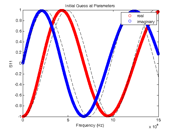
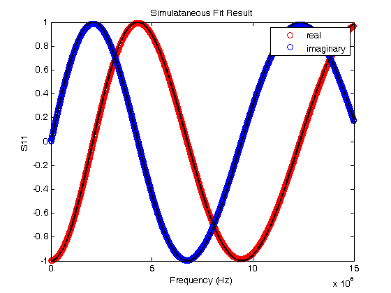
% Jake Bobowsk
% July 26, 2017
% Created using MATLAB R2014a

clearvars;
format longE;

% Sometimes a two sets of experimental data depend on the same model
% parameters.  Consider, for example, the LRC resonator.  One could measure
% both the magnitude and phase of the voltage across the resistor as a
% function of frequency.  Both of these quantities depend on the resonant
% frequency of the system and a loss parameter.  The magnitude and phase
% data could be fit independently to determine two sets of the parameters.
% Perhaps you could then take a weighted average of the results to produce
% a single 'best' value for the resonant frequency and loss parameter.
% However, a better approach is to simultaneously fit the two data sets and
% directly extract a single best-fit value for each parameter.  This
% tutorial shows you how to implement a simultaneous fits to multiple data
% sets that, each having their own model, but sharing at least some of the
% same best-fit parameters.

% This tutorial makes use of a MATLAB script called 'nlinmultifit.m' which
% was created by Chen Avinadav.  I will not make an attempt to explain his
% code, but below are the comments provided by the author at the beginning
% of his script:

%NLINMULTIFIT Nonlinear least-squares regression of multiple data sets
%
%	A wrapper function for NLINFIT which allows simulatenous fitting of
%	multiple data sets with shared fitting parameters. See example below.
%
%	Unlike different solutions (using fminsearch or similar functions)
%	this approach enables simple estimation of model predictions and
%	their confidence intervals, as well as confidence intervals on the
%	fitted parameters (using the built-in NLPREDCI and NLPARCI functions).
%
%	INPUT:
% 		x_cell,y_cell: Cell arrays containing the x,y vectors of the fitted
%					   data sets.
% 		mdl_cell: Cell array containing model functions for each data set.
% 		beta0: Vector containing initial guess of the fitted parameters.
% 		options: Structure containing control parameters for NLINFIT (see
%				 help file on NLINFIT for more details).
%		Name,Value pairs: additional options passed to NLINFIT (see help
%						  file on NLINFIT for more details). The 'Weights'
%						  input option may be specified as a cell array,
%						  similar to the input of x_cell and y_cell.
%
%	NOTE:
%		Unless a cell array of weights is explicitly given, NLINMULTIFIT
%		will create a weights vector such that all points in all datasets
%		receive equal weight regardless of each dataset length.
%
%
%	OUTPUT:
%		beta,r,J,Sigma,mse,errorparam,robustw: Direct output from NLINFIT.
%
%	EXAMPLE:
% 		% Generate X vectors for both data sets
% 		x1 = 0:0.1:10;
% 		x2 = 0:1:10;
%
% 		% Generate Y data with some noise
% 		y1 = cos(2*pi*0.5*x1).*exp(-x1/5) + 0.05*randn(size(x1));
% 		y2 = 0.5 + 2*exp(-(x2/5)) + 0.05*randn(size(x2));
%
% 		% Define fitting functions and parameters, with identical
%		% exponential decay for both data sets
% 		mdl1 = @(beta,x) cos(2*pi*beta(1)*x).*exp(-x/beta(2));
% 		mdl2 = @(beta,x) beta(4) + beta(3)*exp(-(x/beta(2)));
%
% 		% Prepare input for NLINMULTIFIT and perform fitting
% 		x_cell = {x1, x2};
% 		y_cell = {y1, y2};
% 		mdl_cell = {mdl1, mdl2};
% 		beta0 = [1, 1, 1, 1];
% 		[beta,r,J,Sigma,mse,errorparam,robustw] = ...
%					nlinmultifit(x_cell, y_cell, mdl_cell, beta0);
%
% 		% Calculate model predictions and confidence intervals
% 		[ypred1,delta1] = nlpredci(mdl1,x1,beta,r,'covar',Sigma);
% 		[ypred2,delta2] = nlpredci(mdl2,x2,beta,r,'covar',Sigma);
%
% 		% Calculate parameter confidence intervals
% 		ci = nlparci(beta,r,'Jacobian',J);
%
% 		% Plot results
% 		figure;
% 		hold all;
% 		box on;
% 		scatter(x1,y1);
% 		scatter(x2,y2);
% 		plot(x1,ypred1,'Color','blue');
% 		plot(x1,ypred1+delta1,'Color','blue','LineStyle',':');
% 		plot(x1,ypred1-delta1,'Color','blue','LineStyle',':');
% 		plot(x2,ypred2,'Color',[0 0.5 0]);
% 		plot(x2,ypred2+delta2,'Color',[0 0.5 0],'LineStyle',':');
% 		plot(x2,ypred2-delta2,'Color',[0 0.5 0],'LineStyle',':');
%
%	AUTHOR:
%		Chen Avinadav
%		mygiga (at) gmail
%

% In the example below, the signal reflected (S11) from a short section of
% coaxial cable terminated by an inductive loop was measured.  S11 has both
% real and imaginary components that depend on the same set of parameters.
% We will simulataneously fit the real and imaginary parts to their
% respective models and extract a single set of best fit parameters.

% Import the data and plot it.  The data file has three columns: 1. frequency, 2. real
% component of S11, and 3. imaginary component of S11.
M = dlmread('S11 - real imag.dat');
fdata = M(:,1)';
Sreal = M(:,2)';
Simag = M(:,3)';
plot(fdata, Sreal, 'or');
hold on;
plot(fdata, Simag, 'ob');

xlabel('Frequency (Hz)');
ylabel('S11');
title('Initial Guess at Parameters');
legend('real','imaginary')

% Here we define some quantities that will be needed.
% Z0 is the characteristic impedance of the coaxial cable.
% L1 is a guess at the inductance of the loop at the end of the cable
% q is a time that is determined by the speed of light, the length of the
% coaxial cable, and the dielectric constant of the insulator between the
% inner and outer conductors of the cable.  Again, I'm making a guess at
% its value.
% When we do the fits, L1 and q will be the common fit parameters shared by
% the models of the real and imaginary parts of the reflection coefficient
% S11.
Z0 = 50; % ohms
L1 = 0.2e-9; % henries
q =3.2e-9; % seconds

% Xin is an expression for the reactance of the lenght of coaxial cable
% terminated by a loop of inductance L1.
Xin = Z0*(2*pi*fdata*L1/Z0 + tan(q*fdata))./(1-(2*pi*fdata*L1/Z0).*tan(q*fdata));

% Here are the models for the real and imaginary parts of S11.
S11real = ((Xin/Z0).^2-1)./((Xin/Z0).^2+1);
S11imag = 2*(Xin/Z0)./((Xin/Z0).^2+1);

% Before starting the fit routine, we'll plot the model on top of the data
% to see if your guesses at the values of L1 and q are reasonable.  If
% they're not too bad, we'll use them at the initial parameters at the
% start of the fit.
plot(fdata, S11real, '--k');
plot(fdata, S11imag, '--k');
hold off;

% Let's clear everything and start setting up for the simulataneous fit.
clearvars;
format longE;

% Import the data.
M = dlmread('S11 - real imag.dat');
fdata = M(:,1)';
Sreal = M(:,2)';
Simag = M(:,3)';
figure();
plot(fdata,Sreal,'or');
hold on;
plot(fdata,Simag,'ob');

xlabel('Frequency (Hz)');
ylabel('S11');
title('Simulataneous Fit Result');
legend('real','imaginary')

% To do the fitting, we will rely on the nlinmultifit.m script.  The
% nlinmultifit.m script must be placed in the same directory as script that
% we are currently working in (simultaneous_fits.m)

% When we execute nlinmultifit, we will have to pass to it the x and y data
% for each of our data sets.  We will pass two vectors each for x and y.
% These vectors will be stored in "cells".  Curly braces are used to
% construct cells.  In our example, the two datasets have the same x
% values, so we enter fdata twice in the x_cell.  The y_cell has the real
% and imaginary S11 values.  If you wanted to simultaneously fit to three
% or more datasets, you would just have to enter the correct number of row
% vectors in each of the two cells.
x_cell = {fdata, fdata};
y_cell = {Sreal, Simag};

% We now define our model functions.
% Z0 = 50 ohms is a constant (the characteristic impedance of the coaxial
% cable.
% f is defined as a variable.  It represents frequency, our independent
% variable.
% Our model will have two parameters:
% b(1) = L1 is the inductance of the loop at the end of the coaxial cable.
% b(2) = q is a time determined by the length l of the coaxial cable, the
% speed of light c, and the dielectric constant e of the insulator filling
% the space between the inner and outer conductors [q = 2l/(c/sqrt(e))]
Z0 = 50;
syms f
b = sym('b', [1 2]);

% These next few steps are, admittedly, a bit tricky.  Like in the nonlinear fit
% tutorial, we need to define our fit models as functions.  It took me
% quite a while to figure out a way to make this work...

% First, just enter the models as regular functions.  Remember, b(1)
% represents L1 and b(2) represents q.  Also, any time you need to divide
% by a vector or raise a vector to a power, put a dot (.) in front of the
% operator.  This tells MATLAB that the operation should be performed
% element by element rather than using some kind of vector product.
% Notice also that I have scaled b(1) by 1e-9.  This has been done so that
% L1 will be determined in units of nanohenries.  b(2) has been scaled by
% the same factor so that q will be determined in units of nanoseconds.  I
% have done this so that b(1) and b(2) will come out to be on the order of
% 1 or 10 (0.1 would be okay too).  In general, it is good practice to
% scale your fit parameters so that they will not be too different.  i.e.
% you don't want the fit routine to have to deal with one parameter that is
% on the order of 1e6 and another that is 1e-12.  I always try to get my
% fit parameters to come out to be between 0.1 and 10.
Xin = Z0*(2*pi*f*b(1)*1e-9/Z0 + tan(b(2)*1e-9*f))./(1-(2*pi*f*b(1)*1e-9/Z0).*tan(b(2)*1e-9*f));
S11real = ((Xin/Z0).^2-1)./((Xin/Z0).^2+1);
S11imag = 2*(Xin/Z0)./((Xin/Z0).^2+1);

% Here's the bit that took me will to work out...
% matlabFunction converts our S11real expression into a function of b1, b2,
% and f.  Unfortunately, the nonlinear fit routine requirs a function of a
% vector b and scalar f. The @(b,f) line converts our function of three
% scalars (b1, b2, and f) into a function of vector b and scalar f.  b is a
% tow-component vector.  The first component is b(1) (i.e. L1) and the
% second component is b(2) (i.e q).
S11Rfcn = matlabFunction(S11real);
mdlreal = @(b,f) S11Rfcn(b(1), b(2), f);

% Do the same to construct the model function for the imaginary component
% of S11.
S11Ifcn = matlabFunction(S11imag);
mdlimag = @(b,f) S11Ifcn(b(1), b(2), f);

% Just like we made cells for the x and y data, we make a cell of the model
% functions.
mdl_cell = {mdlreal, mdlimag};

% beta0 is vector of initial guesses at the two parameters L1 and q,
% respectively.  We use the values from the plots that we generated right
% at the start of this tutorial.  We know that the guesses aren't perfect,
% but hopefully they'll be good enough.  If not, we'll have to try another
% set of guesses...
beta0 = [0.2, 3.2];

% In the data used in this tutorial, all data points are going to be
% weighted equally (i.e. there's no great variation in the y uncertainties
% as frequency is swept).  However, in general you would have y
% uncertainties for each set of data that would be changing in some way.
% In that case, you should define weights for each dataset that are
% determined from one over the square of the y uncertainties.  Then you
% would construct a weights cell.

% To demonstrate the use of weights, I define two weights vectors in which
% all elements are one, i.e. equally weighted points.  Then, I make the
% weights cell called w_cell
weights1 = ones(1, length(fdata));
weights2 = ones(1, length(fdata));
w_cell = {weights1, weights2};

% Finally, here is where we call nlinmultifit.m to do the simultaneous
% fits.  To nlinmultifit, we pass x_cell, y_cell, mdl_cell, beta0 (the
% initial guess at the parameters), we use the 'Weights' option, and then
% pass w_cell.
[beta,r,J,Sigma,mse,errorparam,robustw] = ...
					nlinmultifit(x_cell, y_cell, mdl_cell, beta0, 'Weights', w_cell);

% If you didn't want to do a weighted fit, you could just implement nlinmultifit as follows:
% [beta,r,J,Sigma,mse,errorparam,robustw] = ...
%					nlinmultifit(x_cell, y_cell, mdl_cell, beta0);

% These next two lines are used to calculate model predictions.
[ypred1,delta1] = nlpredci(mdlreal,fdata,beta,r,'covar',Sigma);
[ypred2,delta2] = nlpredci(mdlimag,fdata,beta,r,'covar',Sigma);

% We can now plot the best-fit results with the original data.
plot(fdata,ypred1,'Color','k','LineWidth',2);
plot(fdata,ypred2,'Color','k','LineWidth',2);
hold off;
% The fits look very good!

% Here are the calculations of parameter 95% confidence intervals.
ci = nlparci(beta,r,'Jacobian',J);

% To estimate the best-fit parameters, I take the average of the confidence
% bounds.  I use have the difference of the confidence bounds to estimate
% the uncertainty in the best-fit parameters.
L1 = (ci(1,2) + ci(1,1))/2 % nH
dL1 = (ci(1,2) - ci(1,1))/2 % nH
q = (ci(2,2) + ci(2,1))/2 % ns
dq = (ci(2,2) - ci(2,1))/2 % ns

% L1 = 11.995 +/- 0.017 nH
% q = 2.3131 +/- 0.0007 ns
L1 =

     1.199497925822889e+01


dL1 =

     1.736682191388006e-02


q =

     2.313058330242801e+00


dq =

     6.960790543395490e-04